How to Install and Secure MariaDB on RHEL 8: Step-by-Step Guide

 How to Install and Secure MariaDB on RHEL 8: Step-by-Step

Introduction

MariaDB is a popular open-source database management system, often chosen for its speed, reliability, and open development model. If you're working with Red Hat Enterprise Linux (RHEL) 8 and want to set up a MariaDB server, . This guide will walk you through the complete installation process of MariaDB on RHEL 8, from adding the necessary repositories to securing your database server.

Preparing Your RHEL 8 System

Before installing MariaDB, ensure your system is up-to-date to avoid compatibility issues and have the latest security patches.

Step 1: Update Your System

Run the following command to update all packages:

sudo dnf update -y

Updating your system ensures that you're starting from a clean and secure environment.

---

2. Adding the Official MariaDB Repository

RHEL 8's default package repositories do not always contain the latest version of MariaDB. Adding the official MariaDB repository allows you to install and update MariaDB easily.

Step 2: Create a MariaDB Repository File

1. Create a new repo file for MariaDB in /etc/yum.repos.d/.

   sudo  /etc/yum.repos.d/MariaDB.repo <<EOF
   [mariadb]
   name = MariaDB
   baseurl = http://yum.mariadb.org/10.5/rhel8-amd64
   gpgkey=https://yum.mariadb.org/RPM-GPG-KEY-MariaDB
   gpgcheck=1
   EOF
   

   Replace 10.5 with the version of MariaDB you wish to install. You can check the MariaDB download page for available versions.

2. Import the GPG Key To verify the packages, import MariaDB’s official GPG key:

   
   sudo rpm --import https://yum.mariadb.org/RPM-GPG-KEY-MariaDB
   

---

3. Installing MariaDB

Now that the repository is added, you can proceed with the installation of the MariaDB server and client.

Step 3: Install MariaDB Server and Client

sudo dnf install -y MariaDB-server MariaDB-client

The -y flag automatically answers "yes" to prompts during the installation process.

---

4. Starting and Enabling MariaDB Service

Once MariaDB is installed, the next step is to start and enable it so it automatically starts on boot.

Step 4: Start the MariaDB Service

sudo systemctl start mariadb

This starts the MariaDB server, which will now be running in the background.

Step 5: Enable MariaDB to Start on Boot

sudo systemctl enable mariadb

Enabling MariaDB ensures that it starts automatically whenever your system boots.

Step 6: Verify the Service Status

To confirm that MariaDB is active and running, use the following command:

sudo systemctl status mariadb

---

5. Securing the MariaDB Installation

It’s crucial to secure your MariaDB installation by setting a root password, removing anonymous users, and restricting remote root access.

Step 7: Secure MariaDB with mysql_secure_installation

sudo mysql_secure_installation

During this process, you will be prompted to:

• Set a strong root password.
• Remove anonymous users.
• Disallow root login remotely.
• Remove test databases and access to them.
• Reload privilege tables to apply changes.

Answer the prompts as recommended to harden your MariaDB installation.

---

6. Verifying the Installation

After securing your installation, confirm that MariaDB is properly installed and configured.

Step 8: Access the MariaDB Shell

sudo mysql -u root -p

You’ll be prompted for the root password you set during the mysql_secure_installation process.

Step 9: Check the MariaDB Version

Once inside the MariaDB shell, run the following command to verify the version:

SELECT VERSION();

Step 10: Exit the MariaDB Shell

exit;

---

7. Configuring Firewall for MariaDB Access

If your RHEL system uses firewalld, you'll need to open port 3306 for MariaDB to allow external connections.

Step 11: Allow MariaDB Through the Firewall

sudo firewall-cmd --permanent --zone=public --add-service=mysql
sudo firewall-cmd --reload

These commands allow traffic on port 3306, which is MariaDB's default port.

Step 12: Verify Firewall Rules

sudo firewall-cmd --list-all

This confirms that the mysql service is allowed through the firewall.

---

8. Configuring MariaDB for Optimal Performance

MariaDB's configuration file is typically located at /etc/my.cnf.d/mariadb-server.cnf. For optimal performance, you may need to make adjustments based on your server's specifications and the workload.

Step 13: Edit the Configuration File

sudo nano /etc/my.cnf.d/mariadb-server.cnf

Step 14: Recommended Settings for Better Performance

Add or modify the following parameters in the [mysqld] section:

[mysqld]
bind-address = 0.0.0.0                # Allow remote connections
max_connections = 200                 # Adjust as per your application needs
innodb_buffer_pool_size = 1G          # Set to 60-80% of server memory for InnoDB
innodb_log_file_size = 256M           # Optimize based on write load
character-set-server = utf8mb4        # Use UTF-8 encoding for broad compatibility
collation-server = utf8mb4_general_ci

Step 15: Restart MariaDB to Apply Changes

sudo systemctl restart mariadb

---

9. Creating a Test Database and User

It’s a good idea to create a test database and user to confirm everything is working as expected.

Step 16: Create a Test Database and User

1. Login to MariaDB

   sudo mysql -u root -p

2. Create a Database

   CREATE DATABASE test_db;

3. Create a User and Grant Privileges

   CREATE USER 'test_user'@'localhost' IDENTIFIED BY 'secure_password';
   GRANT ALL PRIVILEGES ON test_db.* TO 'test_user'@'localhost';
   FLUSH PRIVILEGES;
   

4. Exit the MariaDB Shell

   exit;

---

10. Test the New User Access

You can test access to the new database using the newly created user:

mysql -u test_user -p -D test_db

Enter the password set for test_user to confirm that you can access the test_db database.

Comparison of MariaDB and MySQL

 Comparison of MariaDB and MySQL

This table summarizes the key differences between MariaDB and MySQL, covering aspects like development philosophy, licensing, features, and performance.

 

Daily DBA Scripts for MariaDB

 MariaDB: Essential DBA Practices for Daily Operations

Introduction

MariaDB, a popular open-source relational database, offers high performance, flexibility, and scalability. However, managing a MariaDB database on a day-to-day basis requires constant vigilance and optimization. As a Database Administrator (DBA), having a toolkit of scripts and monitoring techniques is crucial to ensure that your database runs smoothly and efficiently.

In this post, we'll explore essential MariaDB scripts, DBA best practices, and performance tips that can help you maintain and optimize your database operations.

---

Daily DBA Scripts for MariaDB

A DBA’s daily tasks include health checks, performance monitoring, backup routines, and identifying optimization opportunities. Below are some of the fundamental scripts to make your daily operations smooth and manageable.

1. Checking Database Health and Status

To start your day as a DBA, you should quickly check the health and status of your MariaDB server. This provides a snapshot of uptime, connections, and overall performance.

SHOW GLOBAL STATUS;
SHOW VARIABLES LIKE 'version';
SHOW VARIABLES LIKE 'uptime';
SHOW VARIABLES LIKE 'max_connections';

The above script provides details like server version, uptime, and the maximum number of connections, ensuring everything is functioning properly.

---

2. Monitoring Connections and Load

Active connections and thread status directly impact the performance and availability of your database. Monitoring these metrics helps to identify potential overloading issues.

SHOW STATUS LIKE 'Threads%';
SHOW STATUS LIKE 'Connections';
SHOW STATUS LIKE 'Aborted_connects';

By keeping an eye on threads and connections, you can anticipate potential bottlenecks and avoid system overloads.

---

3. Identifying and Optimizing Slow Queries

One of the most significant tasks for a DBA is identifying slow queries that could degrade the performance of your database.

Enable and Monitor the Slow Query Log:

SET GLOBAL slow_query_log = 'ON';
SET GLOBAL long_query_time = 1; -- Log queries taking longer than 1 second
SHOW GLOBAL STATUS LIKE 'Slow_queries';

Slow queries are a major factor in database performance issues. Regularly reviewing and optimizing these queries can greatly improve overall efficiency.

---

4. Monitoring Database and Table Sizes

Understanding the size and growth rate of your tables and databases helps manage storage and allows for capacity planning.

SELECT table_schema AS 'Database', 
       ROUND(SUM(data_length + index_length) / 1024 / 1024, 2) AS 'Size (MB)'
FROM information_schema.tables
GROUP BY table_schema
ORDER BY SUM(data_length + index_length) DESC;

This script helps identify the largest databases and tables, helping you manage disk space effectively.

---

5. Checking Index Usage and Efficiency

Indexes are vital for efficient data retrieval. Monitoring and analyzing index usage ensure your queries are running as fast as possible.

SHOW INDEX FROM your_table_name;

Regularly reviewing indexes allows you to ensure that they are being used correctly and that the correct columns are indexed for your query patterns.

---

6. Viewing Running Queries and Processes

Keeping an eye on currently running queries helps identify and troubleshoot long-running processes.

SHOW FULL PROCESSLIST;

If you find a problematic query, you can terminate it using its process ID:

KILL query_id;

This is particularly useful when a query is blocking resources or taking too long to execute.

---

7. Monitoring and Managing Replication

If your environment uses replication, it is crucial to check its status to ensure that data is being replicated correctly and timely.

SHOW SLAVE STATUS\G
SHOW MASTER STATUS;

Monitoring replication helps maintain data consistency and availability in a distributed setup.

---

8. Regular Backups for Data Protection

Backing up databases is one of the most critical tasks for a DBA. An automated daily backup script ensures that your data is safe.

#!/bin/bash

USER="root"
PASSWORD="your_password"
BACKUP_DIR="/backup/mariadb"
DATE=$(date +%Y%m%d)

mkdir -p "$BACKUP_DIR"
mysqldump -u "$USER" -p"$PASSWORD" --all-databases > "$BACKUP_DIR/all_databases_$DATE.sql"

Make sure to schedule this script using cron jobs or any other scheduling tool to have daily backups ready for disaster recovery.

---

9. Reviewing User Privileges

Ensuring proper user access helps maintain security and prevents unauthorized access to critical data.

SELECT user, host, db, table_name, column_name, privilege_type 
FROM information_schema.column_privileges;

Following the principle of least privilege ensures that users only have the access necessary for their roles.

---

Performance Tips for Monitoring and Optimization

To maintain a high-performance MariaDB environment, active monitoring and optimization are required. Here are some tips to help improve database performance:

1. Use EXPLAIN for Query Optimization

Before executing a query, use EXPLAIN to understand how MariaDB processes it. This allows you to make necessary optimizations.

EXPLAIN SELECT * FROM your_table WHERE column = 'value';

If you see ALL in the type column, it indicates a full table scan, which is a performance red flag. Use indexing and query refactoring to improve performance.

---

2. Set Up Alerts for Critical Performance Metrics

Use monitoring tools like Nagios, Zabbix, or built-in MariaDB monitoring tools to set up alerts for:

• High CPU load
• Memory usage spikes
• Disk I/O saturation
• Slow queries exceeding a threshold

Proactive alerting ensures you can address issues before they affect users.

---

3. Enable Query Caching (If Applicable)

MariaDB offers query caching to speed up frequently executed, unchanged queries.

SET GLOBAL query_cache_size = 16M; -- Enable with size
SET GLOBAL query_cache_type = 'ON';

Monitor cache efficiency:

SHOW STATUS LIKE 'Qcache%';

Note: Query cache is effective only when queries and data don’t change frequently.

---

4. Monitor and Rotate Logs

Regularly monitor log files to track query performance, errors, and general database activity.

cat /var/log/mysql/error.log

Rotate logs using logrotate to prevent disk space issues:

FLUSH LOGS;

---

5. Regularly Optimize Tables

Defragmenting tables by running OPTIMIZE TABLE can help improve performance and reclaim unused space.

OPTIMIZE TABLE your_table_name;

Regularly running OPTIMIZE TABLE on frequently updated tables can enhance performance.

---

6. Leverage Performance Schema for Advanced Monitoring

The Performance Schema provides in-depth metrics about resource usage, memory, and locking.

SET GLOBAL performance_schema = 'ON';
SELECT * FROM performance_schema.events_statements_current;

By leveraging this schema, you can track down performance bottlenecks at a more granular level.

---

Conclusion

As a MariaDB DBA, the health, performance, and security of your database are in your hands. The scripts and best practices provided in this guide will help you proactively manage your database, maintain optimal performance, and prepare for any issues that may arise. Remember, constant monitoring and optimization are key to a well-managed MariaDB environment.

OCI - Setting Up a Virtual Cloud Network (VCN)

 Setting Up a Virtual Cloud Network (VCN) in Oracle Cloud: A Step-by-Step

Introduction

A Virtual Cloud Network (VCN) is a fundamental building block in Oracle Cloud Infrastructure (OCI). It’s a private network that you define and control, allowing you to securely connect your cloud resources. This guide will walk you through the process of setting up a VCN in OCI, ensuring that your cloud environment is configured for optimal performance and security.

What is a Virtual Cloud Network (VCN)?

A Virtual Cloud Network (VCN) is a customizable and private network that resides within Oracle Cloud Infrastructure. It provides the foundation for hosting your compute instances, databases, and other resources. By setting up a VCN, you can control your IP addresses, subnets, route tables, and gateways, enabling secure communication within your cloud environment and with external networks.

Key Components of a VCN

• Subnets: These are segments within your VCN where you can launch OCI resources, such as compute instances.
• Route Tables: These define how traffic flows between subnets and external networks.
• Gateways: Gateways, such as Internet Gateways and NAT Gateways, enable communication between your VCN and external networks.
• Security Lists and Network Security Groups (NSGs): These control the inbound and outbound traffic to your resources.

Step 1: Creating a VCN

To start, you'll need to create a VCN in your OCI environment. Here’s how:

1. Navigate to the Networking Service:

   • From the OCI dashboard, click on "Networking" and then "Virtual Cloud Networks."

2. Create a New VCN:

   • Click on "Create VCN" to start the setup.
   • Name Your VCN: Give your VCN a meaningful name that reflects its purpose.
   • CIDR Block: Specify the IP address range for your VCN using CIDR notation (e.g., 10.0.0.0/16).

3. Create Subnets:

   • Subnets: Create at least one public subnet and one private subnet.
   • Public Subnet: Used for resources that need to communicate with the internet, such as web servers.
   • Private Subnet: Used for resources that do not need direct internet access, such as databases.

4. Configure Route Tables:

   • Default Route Table: Ensure that the route table is configured to allow traffic between subnets and any external gateways.

5. Add Gateways:

   • Internet Gateway: Attach an Internet Gateway if you need internet access for resources in the public subnet.
   • NAT Gateway: For resources in the private subnet that need outbound internet access, attach a NAT Gateway.

6. Create Security Lists or Network Security Groups (NSGs):

   • Security Lists: Configure security lists to allow or deny specific types of traffic to your subnets.
   • NSGs: Alternatively, use NSGs for more granular control over traffic rules for specific resources.

7. Review and Create:

   • Review your VCN configuration and click “Create” to finalize the setup.

Step 2: Associating Resources with Your VCN

Once your VCN is created, you can start associating OCI resources with it:

• Launch Compute Instances: When creating a new compute instance, select the appropriate VCN and subnet.
• Attach Block Storage: Ensure that any block storage you attach to your instances is within the same VCN.
• Configure Load Balancers: If you're using load balancers, place them in the public subnet for internet-facing applications.

Step 3: Managing and Modifying Your VCN

Your network requirements may evolve, so it’s important to know how to manage and modify your VCN:

• Add More Subnets: As your environment grows, you may need to add additional subnets.
• Update Route Tables: Modify route tables to accommodate new network routes or changes in traffic flow.
• Adjust Security Rules: Update your security lists or NSGs to reflect changes in security requirements.

Best Practices for VCN Setup

• Plan Your IP Addressing: Carefully plan your CIDR block and subnet ranges to avoid conflicts and ensure scalability.
• Use Private Subnets: Whenever possible, use private subnets for resources that do not require direct internet access to enhance security.
• Regularly Review Security Rules: Periodically review and update security rules to ensure they align with current security policies.

Conclusion

Setting up a Virtual Cloud Network (VCN) is a critical step in building a secure and scalable environment in Oracle Cloud Infrastructure. By following this guide, you’ll have a solid foundation for hosting your cloud resources, with the flexibility to grow and adapt your network as needed. In the next article, we’ll explore how to deploy and configure an Oracle Autonomous Database within your VCN.

Oracle Cloud Infrastructure (OCI)

 Oracle Cloud Infrastructure (OCI)

Introduction:

Oracle Cloud Infrastructure (OCI) is a comprehensive cloud computing platform that offers a wide range of services, including computing, storage, networking, and databases. Whether you’re a developer, a system administrator, or an IT enthusiast, OCI provides the tools you need to build and run modern applications. This guide is designed to help beginners get started with Oracle Cloud, walking you through the basics of setting up your first OCI environment.

---

1. What is Oracle Cloud Infrastructure (OCI)?

Oracle Cloud Infrastructure is Oracle’s cloud service platform, designed to support modern, cloud-native applications. It provides high-performance compute, storage, networking, and database services in a secure, scalable environment. OCI is known for its robust performance, enterprise-grade security, and flexibility, making it a top choice for businesses of all sizes.

Key Features of OCI:

• Compute Services: Virtual machines, bare metal servers, and Kubernetes clusters.
• Storage Solutions: Block storage, object storage, and file storage.
• Networking: Virtual cloud networks, load balancing, and VPN connectivity.
• Database Services: Oracle Autonomous Database, Oracle Exadata, and Oracle MySQL Database Service.

---

2. Setting Up Your Oracle Cloud Account

Before you can start using OCI, you need to set up an Oracle Cloud account. Follow these steps to get started:

1. Sign Up for an Oracle Cloud Account:

   • Visit the Oracle Cloud website and click on the “Start for free” button.
   • Provide the necessary information, including your email address, name, and payment details. Oracle offers a free tier with limited resources, which is ideal for beginners.

2. Accessing the OCI Console:

   • Once your account is set up, log in to the Oracle Cloud Console.
   • The console is your primary interface for managing OCI resources. It provides a dashboard with quick access to all your services and configurations.

---

3. Understanding OCI’s Core Concepts

Before diving into OCI, it’s important to understand some core concepts:

• Regions and Availability Domains:

  • OCI resources are distributed across multiple regions and availability domains (ADs). A region is a geographic area, while an AD is an isolated data center within a region.
  • This architecture ensures high availability and disaster recovery.

• Tenancy:

  • Your Oracle Cloud account is referred to as a tenancy. It’s a secure and isolated partition within OCI where you create and manage resources.

• Compartments:

  • Compartments are logical groups within your tenancy that help you organize and control access to resources. Think of them as folders for your cloud resources.

---

4. Launching Your First Compute Instance

Let’s create a basic compute instance to familiarize ourselves with the process:

1. Navigate to Compute Services:

   • In the OCI Console, select “Compute” from the main menu and click on “Instances.”

2. Create a New Instance:

   • Click on “Create Instance” and provide a name for your instance.
   • Choose an image (Oracle Linux is recommended for beginners) and select a shape (the instance type and resources).

3. Configure Networking:

   • Select or create a Virtual Cloud Network (VCN) and a subnet.
   • You can use the default VCN or create a new one for better control.

4. Launch the Instance:

   • Review your settings and click “Create.” Your instance will launch in a few minutes.
   • Once the instance is running, you can connect to it using SSH and start deploying applications.

---

5. Managing and Scaling Your Resources

As your needs grow, OCI allows you to scale your resources easily:

• Scaling Compute Instances:

  • You can scale your compute instances up or down by changing the shape or adding more instances.

• Adding Storage:

  • Attach additional block storage volumes to your compute instances for extra storage.

• Load Balancing:

  • Use the OCI Load Balancer service to distribute traffic across multiple instances, ensuring high availability.

---

Conclusion:

Starting with Oracle Cloud Infrastructure is straightforward, and with a basic understanding of its core concepts, you can quickly deploy and manage your first cloud resources. 

Understanding the EBS_SYSTEM Schema in Oracle E-Business Suite R12

EBS_SYSTEM Schema in Oracle E-Business Suite R12

Introduction

Oracle E-Business Suite (EBS) R12 has introduced several innovations to improve system performance and availability. One of the critical components in this version is the EBS_SYSTEM schema, which plays a pivotal role in the online patching process. In this blog, we'll explore what the EBS_SYSTEM schema is, its functions, and why it's essential for maintaining an efficient and secure EBS environment.

What is the EBS_SYSTEM Schema?

The EBS_SYSTEM schema is a dedicated database user introduced in EBS R12.2 to support the online patching functionality. It isolates patching operations from the main application users, ensuring that patches can be applied with minimal downtime.

Key Roles and Responsibilities

1. Online Patching (ADOP)

The primary role of the EBS_SYSTEM schema is to manage and execute online patching processes. This includes creating and managing patch editions, synchronizing data between editions, and ensuring that changes are applied without affecting the live environment.

2. Security and Isolation

By using a separate schema for patching operations, EBS_SYSTEM enhances the security and stability of the EBS environment. This segregation ensures that only authorized operations can be performed during the patching process.

3. Patch Edition Management

The EBS_SYSTEM schema is responsible for handling patch editions. When a patch cycle is initiated, EBS_SYSTEM manages the creation of a new patch edition and synchronizes it with the running edition.

4. Data Synchronization

It ensures that all data changes made in the patch edition are correctly propagated to the run edition during the finalization phase, maintaining data consistency and integrity.

5. Object Editioning

EBS_SYSTEM manages editioned objects, allowing different definitions of the same object in different editions. This capability is crucial for applying patches without disrupting the current production environment.

How the EBS_SYSTEM Schema Works

Prepare Phase

During the adop phase=prepare, the EBS_SYSTEM schema sets up the patch edition and synchronizes it with the run edition, preparing the environment for patch application.

Apply Phase

In the adop phase=apply, the schema applies the patches to the patch edition. This ensures that all changes are made in a controlled environment, separate from the live production system.

Finalize and Cutover Phases

During the adop phase=finalize, EBS_SYSTEM checks and prepares the system for switching to the new edition. The adop phase=cutover then makes the patch edition the new run edition, minimizing downtime.

Cleanup Phase

Finally, the adop phase=cleanup removes any obsolete objects and data from previous editions, ensuring that the system remains clean and efficient.

Security Considerations

Given its critical role, the EBS_SYSTEM schema must be secured properly. Ensure strong password policies, monitor its activities regularly, and restrict excessive privileges to prevent unauthorized access and potential security breaches.

Benefits of Using the EBS_SYSTEM Schema

1. Reduced Downtime: By managing patches in a separate edition, the schema allows patches to be applied with minimal disruption to users.
2. Enhanced Security: Isolating patch operations enhances the security and integrity of the EBS environment.
3. Improved Efficiency: Automating patch management tasks reduces the manual effort required from DBAs, leading to faster and more efficient patching processes.

Conclusion

The EBS_SYSTEM schema is a vital component of Oracle E-Business Suite R12, facilitating seamless and secure online patching. Understanding its roles and responsibilities helps DBAs and system administrators maintain a robust and efficient EBS environment. By leveraging the capabilities of EBS_SYSTEM, organizations can ensure minimal downtime, enhanced security, and optimized performance during patching operations.

ASM QUERIES

ASM DISK SPACE REPORT

set lines 255

col path for a35

col Diskgroup for a15

col DiskName for a25

col disk# for 999

col total_mb for 999,999,999

col free_mb for 999,999,999

compute sum of total_mb on DiskGroup

compute sum of free_mb on DiskGroup

break on DiskGroup skip 1 on report -

 set pages 255

select a.name DiskGroup, b.disk_number Disk#, b.name DiskName, 

   b.total_mb, b.free_mb, 

   -- b.path, 

   b.header_status

from v$asm_disk b, v$asm_diskgroup a

where a.group_number (+) =b.group_number

order by b.group_number, b.disk_number, b.name;

DISK GROUP USAGE

set lines 120

col "Redundancy" for a15

col "Diskgroup" for a12

select a.name "Diskgroup" , round(sum(b.total_mb)/1024,1) "Size GB",  

       round(sum(b.free_mb)/1024,1) "Free GB", 

       decode (a.type, 'EXTERN',round(sum(b.free_mb)/1024,1),'NORMAL',round(sum(b.free_mb)/1024/2,1),'HIGH',round(sum(b.free_mb)/1024/3,1))  "Usable GB", 

       decode (a.type, 'EXTERN',round(sum(b.free_mb)/1024/1024,1),'NORMAL',round(sum(b.free_mb)/1024/1024/2,1),'HIGH',round(sum(b.free_mb)/1024/1024/3,1))  "Usable TB", 

       round((sum(b.total_mb)-sum(b.free_mb))/sum(b.total_mb)*1000)/10 "Use%",

       a.type "Redundancy"

from v$asm_disk b, v$asm_diskgroup a 

where  a.group_number (+) =b.group_number 

group by a.name, a.type order by 1;

GROUP BY USAGE

set pages 100

col database for a15

SELECT NVL(dbname, '-- TOTAL') database, round(SUM(space)/1024/1024) mb_used, 

       round(SUM(space) / AVG(total_mb * 1024 * 1024) * 100, 2) pct_used

FROM (

  SELECT gname, file_type, space, aname, system_created, alias_directory,

         regexp_substr(full_alias_path, '[[:alnum:]_]*',1,4) dbname, total_mb

    FROM (

      SELECT system_created, alias_directory, file_type,space, level, gname, aname,

          concat('+'||gname, sys_connect_by_path(aname, '/')) full_alias_path, total_mb

        FROM (

          SELECT b.name gname, b.total_mb, a.parent_index pindex, a.name aname,

                 a.reference_index rindex, a.system_created, a.alias_directory,

                 c.type file_type, c.space

            FROM v$asm_alias a 

            JOIN v$asm_diskgroup b ON a.group_number = b.group_number

       LEFT JOIN v$asm_file c ON a.group_number = c.group_number

             AND a.file_number = c.file_number

             AND a.file_incarnation = c.incarnation

        ) START WITH (mod(pindex, power(2, 24))) = 0 AND rindex IN (

          SELECT a.reference_index FROM v$asm_alias a, v$asm_diskgroup b

           WHERE a.group_number = b.group_number

             AND (mod(a.parent_index, power(2, 24))) = 0

        ) CONNECT BY prior rindex = pindex

    ) WHERE NOT file_type IS NULL AND system_created = 'Y' )

GROUP BY ROLLUP (dbname)

/

                                                    

Oracle ASM USAGE

select name, total_mb, free_mb, 

       round(100*(total_mb-free_mb)/greatest(1,total_mb),0) as used_pct 

  from v$asm_diskgroup;

A key difference between TP and TPURGENT

Difference between TP and TPURGENT TP

When you are using Autonomous Transaction Processing database, as well as the LOW, MEDIUM and HIGH services that are also present on the Autonomous Data Warehouse offering, there are TP and TPURGENT services that you can use. Difference  as you can see below:

SQL> select plan, group_or_subplan, cpu_p1
  2  from DBA_RSRC_PLAN_DIRECTIVES
  3  where group_or_subplan like '%TP%';

PLAN         GROUP_OR_SUB     CPU_P1
------------ ------------ ----------
OLTP_PLAN    TP                    8
OLTP_PLAN    TPURGENT             12

there is another important difference to be aware of. As the name suggests, TP is designed for “transactional processing” which means the expectation is for short, snappy transactions. A consequence of this, is that there is no capacity to perform operations in parallel when connecting to the TP service, even if you try to force it.

SQL> conn ADMIN/xxxx@myatp_tp
Connected.

SQL> create table t as select * from dba_objects;

Table created.

SQL> select owner, count(*) from t group by owner;

OWNER                            COUNT(*)
------------------------------ ----------
SYS                                 19401
SYSTEM                                472
DBSNMP                                 59
APPQOSSYS                               6
...

43 rows selected.

SQL> select * from dbms_xplan.display_cursor();

PLAN_TABLE_OUTPUT
------------------------------------------------------------------------------------------------------
SQL_ID  gupp4rhyp22fz, child number 0
-------------------------------------
select owner, count(*) from t group by owner

Plan hash value: 47235625

-----------------------------------------------------------------------------------
| Id  | Operation                  | Name | Rows  | Bytes | Cost (%CPU)| Time     |
-----------------------------------------------------------------------------------
|   0 | SELECT STATEMENT           |      |       |       |    22 (100)|          |
|   1 |  HASH GROUP BY             |      |    43 |   430 |    22  (14)| 00:00:01 |
|   2 |   TABLE ACCESS STORAGE FULL| T    | 68290 |   666K|    20   (5)| 00:00:01 |
-----------------------------------------------------------------------------------


14 rows selected.

SQL>
SQL> select /*+ parallel */ owner, count(*) from t group by owner;

OWNER                            COUNT(*)
------------------------------ ----------
SYS                                 19401
SYSTEM                                472
DBSNMP                                 59
APPQOSSYS                               6
...

43 rows selected.

SQL> select * from dbms_xplan.display_cursor();

PLAN_TABLE_OUTPUT
----------------------------------------------------------------------------------------------------------------------------------
SQL_ID  caw2nz87gxkja, child number 0
-------------------------------------
select /*+ parallel */ owner, count(*) from t group by owner

Plan hash value: 47235625

-----------------------------------------------------------------------------------
| Id  | Operation                  | Name | Rows  | Bytes | Cost (%CPU)| Time     |
-----------------------------------------------------------------------------------
|   0 | SELECT STATEMENT           |      |       |       |    22 (100)|          |
|   1 |  HASH GROUP BY             |      |    43 |   430 |    22  (14)| 00:00:01 |
|   2 |   TABLE ACCESS STORAGE FULL| T    | 68290 |   666K|    20   (5)| 00:00:01 |
-----------------------------------------------------------------------------------

Hint Report (identified by operation id / Query Block Name / Object Alias):
Total hints for statement: 1 (U - Unused (1))
---------------------------------------------------------------------------

   0 -  STATEMENT
         U -  parallel

Note
-----
   - automatic DOP: Computed Degree of Parallelism is 1


25 rows selected.

SQL>

Compare that to when you connect to the TPURGENT service. By default, just like the TP service operations are expected to the business transactions and thus no parallelism is activated.

SQL> conn ADMIN/xxxx@myatp_tpurgent
Connected.

SQL> create table t as select * from dba_objects;

Table created.

SQL> select owner, count(*) from t group by owner;

OWNER                            COUNT(*)
------------------------------ ----------
SYS                                 19317
SYSTEM                                472
DBSNMP                                 59
APPQOSSYS                               6
...


44 rows selected.

SQL> select * from dbms_xplan.display_cursor();

PLAN_TABLE_OUTPUT
----------------------------------------------------------------------------------------------------------------------------------
SQL_ID  gupp4rhyp22fz, child number 0
-------------------------------------
select owner, count(*) from t group by owner

Plan hash value: 47235625

-----------------------------------------------------------------------------------
| Id  | Operation                  | Name | Rows  | Bytes | Cost (%CPU)| Time     |
-----------------------------------------------------------------------------------
|   0 | SELECT STATEMENT           |      |       |       |    23 (100)|          |
|   1 |  HASH GROUP BY             |      |    44 |   440 |    23  (14)| 00:00:01 |
|   2 |   TABLE ACCESS STORAGE FULL| T    | 71476 |   698K|    21   (5)| 00:00:01 |
-----------------------------------------------------------------------------------


14 rows selected.

However, under TPURGENT you can obtain parallel processing should you need it by explicitly nominating it with hint:

SQL> select /*+ parallel */ owner, count(*) from t group by owner;

OWNER                            COUNT(*)
------------------------------ ----------
SYS                                 19317
SYSTEM                                472
DBSNMP                                 59
APPQOSSYS                               6
...


44 rows selected.

SQL> select * from dbms_xplan.display_cursor();

PLAN_TABLE_OUTPUT
----------------------------------------------------------------------------------------------------------------------------------
SQL_ID  caw2nz87gxkja, child number 1
-------------------------------------
select /*+ parallel */ owner, count(*) from t group by owner

Plan hash value: 129087698

--------------------------------------------------------------------------------------------------------------------------
| Id  | Operation                        | Name     | Rows  | Bytes | Cost (%CPU)| Time     |    TQ  |IN-OUT| PQ Distrib |
--------------------------------------------------------------------------------------------------------------------------
|   0 | SELECT STATEMENT                 |          |       |       |    13 (100)|          |        |      |            |
|   1 |  PX COORDINATOR                  |          |       |       |            |          |        |      |            |
|   2 |   PX SEND QC (RANDOM)            | :TQ10001 |    44 |   440 |    13  (16)| 00:00:01 |  Q1,01 | P->S | QC (RAND)  |
|   3 |    HASH GROUP BY                 |          |    44 |   440 |    13  (16)| 00:00:01 |  Q1,01 | PCWP |            |
|   4 |     PX RECEIVE                   |          |    44 |   440 |    13  (16)| 00:00:01 |  Q1,01 | PCWP |            |
|   5 |      PX SEND HASH                | :TQ10000 |    44 |   440 |    13  (16)| 00:00:01 |  Q1,00 | P->P | HASH       |
|   6 |       HASH GROUP BY              |          |    44 |   440 |    13  (16)| 00:00:01 |  Q1,00 | PCWP |            |
|   7 |        PX BLOCK ITERATOR         |          | 71476 |   698K|    11   (0)| 00:00:01 |  Q1,00 | PCWC |            |
|*  8 |         TABLE ACCESS STORAGE FULL| T        | 71476 |   698K|    11   (0)| 00:00:01 |  Q1,00 | PCWP |            |
--------------------------------------------------------------------------------------------------------------------------

Predicate Information (identified by operation id):
---------------------------------------------------

   8 - storage(:Z>=:Z AND :Z<=:Z)

Note
-----
   - automatic DOP: Computed Degree of Parallelism is 2


29 rows selected.

SQL>

Autonomous Transaction Processing (ATP)

So its important to be aware of the parallelism facilities defined for MEDIUM and HIGH. We’ll do operations in parallel whenever possible. You get faster queries and faster DML but there are implications on the way you write your scripts, the locking that will result and how commit processing must be handled. HIGH and MEDIUM are not just “bigger” versions of the LOW service.

Predefined Database Service Names for Autonomous Transaction

The predefined service names provide different levels of performance and concurrency for Autonomous Transaction Processing.

• tpurgent: The highest priority application connection service for time critical transaction processing operations. This connection service supports manual parallelism.
• tp: A typical application connection service for transaction processing operations. This connection service does not run with parallelism.
• high: A high priority application connection service for reporting and batch operations. All operations run in parallel and are subject to queuing.
• medium: A typical application connection service for reporting and batch operations. All operations run in parallel and are subject to queuing. Using this service the degree of parallelism is limited to four (4).
• low: A lowest priority application connection service for reporting or batch processing operations. This connection service does not run with parallelism.

 For standard transactional activities on ATP, make sure it uses the TP or TPURGENT services. If you need faster performance for volume operations, then HIGH and MEDIUM are your friend, 

but understand the locking and commit implications.

Predefined Database Service Names for Autonomous

 Databases 

Regarding parallelism for different services.

Oracle doc -

https://docs.oracle.com/en-us/iaas/autonomous-database/doc/connecting.html#GUID-07401C82-6A01-4CDF-AAE5-54B78B50CA0A

Ref - Connor Mcdonald ( TP AND TP URGENT )

U

R

GENTA key difference between

 TP and TPURGENT

 ♨️The Fundamental Characteristics of Storage concepts for DBAs.🧩

☑️Conceptual challenges between DBAs and Storage technicians and Developers.

Download and follow the link Below for better understanding 

Storage Concepts

EM 12c, 13c: 'CPU Utilization (%) of a cpu' Metric Showing 'No data to display' On All Metrics In EM Console

 EM 12c, 13c: 'CPU Utilization (%) of a cpu' Metric Showing 'No data to display' On All Metrics In EM Console

Login to OEM Console -> Navigate to the Host target -> Monitoring -> All Metrics -> Expand "CPU Usage" -> Select "CPU Utilization (%) of a CPU" -> Select Last 24 Hours next to "View Data"

Last 24 hours' Graphs Data for the "CPU Utilization (%) of a CPU" metric of Host Target is Not Being Displayed in OEM Cloud Control.

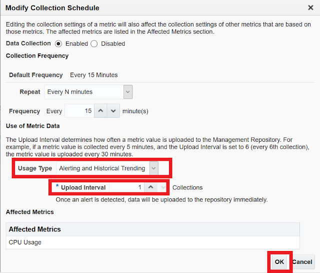
 'Usage Type' of 'Use of Metric Data' is setting "Alerting Only".

⇒This setting means, 'Upload Interval' of this metric is「On Alert].

SOLUTION 

1) Change 'Usage Type' of 'Use of Metric Data' is setting from "Alerting Only" to "Alerting and Historical Trending".

2)'Upload Interval' setting  a value except "0". ※The number must be greater than or equal to 1.

3) Click the "OK" button.

4) Wait for 15 minutes and verify the  EM Console, it will show metrics data.

※It can be changed too, in the following in EM console.

Login to OEM Console -> Navigate to the Host target -> Monitoring -> Metric and Collection Settings -> Edit Collection Settings: <Metric_name>

Document ID - 2630530.1